Manipulating, analyzing, and exporting data with tidyverse

In this lesson we will use tidyverse packages to manipulate and analyze data. We’ll perform similar subsetting processes as before, but with tidyverse tools. Then we’ll exploring linking input and outputs. We’ll also get into the subject of reshaping and formatting data before we end with exporting data.

Data manipulation using `dpylr` and `tidyr`

We’ve learned to subset with brackets [], which is useful, but can become cumbersome with complex subsetting operations. Enter the two packages below, both of which are part of the tidyverse.

dplyr – a package that is useful for tabular data manipulation
tidyr – a package that is useful for donverting between data formats used in plotting / analysis

The tidyverse package tries to address 3 common issues that arise when doing data analysis in R:

The results from a base R function sometimes depend on the type of data.
R expressions are used in a non standard way, which can be confusing for new learners.
The existence of hidden arguments having default operations that new learners are not aware of.

Note

You should have tidyverse installed already. If you do not, you can type the following into the console.

# install the package
install.packages("tidyverse")

# load the package
library("tidyverse")

── Attaching packages ─────────────────────────────────────── tidyverse 1.3.2 ──
✔ ggplot2 3.4.0      ✔ purrr   0.3.5 
✔ tibble  3.1.8      ✔ dplyr   1.0.10
✔ tidyr   1.2.1      ✔ stringr 1.4.1 
✔ readr   2.1.3      ✔ forcats 0.5.2 
── Conflicts ────────────────────────────────────────── tidyverse_conflicts() ──
✖ dplyr::filter() masks stats::filter()
✖ dplyr::lag()    masks stats::lag()

Let’s read in our data using read_csv(), from the tidyverse package, readr.

surveys <- read_csv("~/data-carpentry/data_raw/portal_data_joined.csv") #read in data

Rows: 34786 Columns: 13
── Column specification ────────────────────────────────────────────────────────
Delimiter: ","
chr (6): species_id, sex, genus, species, taxa, plot_type
dbl (7): record_id, month, day, year, plot_id, hindfoot_length, weight

ℹ Use `spec()` to retrieve the full column specification for this data.
ℹ Specify the column types or set `show_col_types = FALSE` to quiet this message.

str(surveys) #inspect the data
view(surveys) #preview the data

Next, we’re going to learn some of the most common dplyr functions

select(): subset columns
filter(): subset rows on conditions
mutate(): create new columns by using information from other columns
group_by() and summarize(): create summary statistics on grouped data
arrange(): sort results
count(): count discrete values

Selecting columns and filtering rows

To select columns of a dataframe, we use select().

select(datafame, columns_to_keep)

select(surveys, plot_id, species_id, weight)

# A tibble: 34,786 × 3
   plot_id species_id weight
     <dbl> <chr>       <dbl>
 1       2 NL             NA
 2       2 NL             NA
 3       2 NL             NA
 4       2 NL             NA
 5       2 NL             NA
 6       2 NL             NA
 7       2 NL             NA
 8       2 NL             NA
 9       2 NL            218
10       2 NL             NA
# … with 34,776 more rows

To EXCLUDE a specific column, put - in front of the variable.

select(surveys, -record_id, -species_id)

# A tibble: 34,786 × 11
   month   day  year plot_id sex   hindfoot…¹ weight genus species taxa  plot_…²
   <dbl> <dbl> <dbl>   <dbl> <chr>      <dbl>  <dbl> <chr> <chr>   <chr> <chr>  
 1     7    16  1977       2 M             32     NA Neot… albigu… Rode… Control
 2     8    19  1977       2 M             31     NA Neot… albigu… Rode… Control
 3     9    13  1977       2 <NA>          NA     NA Neot… albigu… Rode… Control
 4    10    16  1977       2 <NA>          NA     NA Neot… albigu… Rode… Control
 5    11    12  1977       2 <NA>          NA     NA Neot… albigu… Rode… Control
 6    11    12  1977       2 <NA>          NA     NA Neot… albigu… Rode… Control
 7    12    10  1977       2 <NA>          NA     NA Neot… albigu… Rode… Control
 8     1     8  1978       2 <NA>          NA     NA Neot… albigu… Rode… Control
 9     2    18  1978       2 M             NA    218 Neot… albigu… Rode… Control
10     3    11  1978       2 <NA>          NA     NA Neot… albigu… Rode… Control
# … with 34,776 more rows, and abbreviated variable names ¹hindfoot_length,
#   ²plot_type

To choose specific rows based on criteria, we use filter()

filter(surveys, year == 1995)

# A tibble: 1,180 × 13
   record…¹ month   day  year plot_id speci…² sex   hindf…³ weight genus species
      <dbl> <dbl> <dbl> <dbl>   <dbl> <chr>   <chr>   <dbl>  <dbl> <chr> <chr>  
 1    22314     6     7  1995       2 NL      M          34     NA Neot… albigu…
 2    22728     9    23  1995       2 NL      F          32    165 Neot… albigu…
 3    22899    10    28  1995       2 NL      F          32    171 Neot… albigu…
 4    23032    12     2  1995       2 NL      F          33     NA Neot… albigu…
 5    22003     1    11  1995       2 DM      M          37     41 Dipo… merria…
 6    22042     2     4  1995       2 DM      F          36     45 Dipo… merria…
 7    22044     2     4  1995       2 DM      M          37     46 Dipo… merria…
 8    22105     3     4  1995       2 DM      F          37     49 Dipo… merria…
 9    22109     3     4  1995       2 DM      M          37     46 Dipo… merria…
10    22168     4     1  1995       2 DM      M          36     48 Dipo… merria…
# … with 1,170 more rows, 2 more variables: taxa <chr>, plot_type <chr>, and
#   abbreviated variable names ¹record_id, ²species_id, ³hindfoot_length

Connecting inputs and outputs with pipes

We often want to perform multiple manipulations to our datasets. This can be done in a few ways: intermediate steps, nested functions, or pipes.

With intermediate steps, a temporary dataframe is created and used as input into the next function.

surveys2 <- filter(surveys, weight < 5) #filer surveys to create surveys2, the intermediate file
surveys_sml <- select(surveys2, species_id, sex, weight) #use surveys2 as input for the next step

While sometimes useful (for initial validation, etc.), this can clutter the workspace and make it difficult to follow.

Nested functions fit one function inside of another.

surveys_sml <- select(filter(surveys, weight < 5), species_id, sex, weight) # filtering first, then selecting

This is handy, but can be difficult to read if too many functions are nested, as R evaluates the expression from the inside out (in this case, filtering, then selecting).

Pipes (%>%) are a recent addition to R and let you take the output of one function and send it directly to the next function as input. The package enabling this is magrittr, installed when you install dplyr.

surveys %>% # send surveys to filter
  filter(weight < 5) %>% # use surveys as input, filter and send output to select
  select(species_id, sex, weight) # use filtered data as input, select, and send output to console

# A tibble: 17 × 3
   species_id sex   weight
   <chr>      <chr>  <dbl>
 1 PF         F          4
 2 PF         F          4
 3 PF         M          4
 4 RM         F          4
 5 RM         M          4
 6 PF         <NA>       4
 7 PP         M          4
 8 RM         M          4
 9 RM         M          4
10 RM         M          4
11 PF         M          4
12 PF         F          4
13 RM         M          4
14 RM         M          4
15 RM         F          4
16 RM         M          4
17 RM         M          4

Let’s break it down a bit.

We use the pipe to send the surveys dataset through filter()
Filter takes that input, and performs the filtering to keep rows where weight is less than 5, then send the output to select
Select takes that input, and keeps only the species_id, sex, and weight columns.

Note that since %>% takesthe object on its left and passes it as the first argument to the function on its right, we don’t need to explicitly include the data frame as an argument to the filter() and select() functions any more.

Tip

Some may find it helpful to read the pipe like the word “then.” For instance, in the example above, we took the dataframe surveys, then we filtered for rows with weight < 5, then we selected columns species_id, sex, and weight. The dplyr functions by themselves are somewhat simple, but by combining them into linear workflows with the pipe we can accomplish more complex manipulations of dataframes.

If we want to create a new object with this smaller version of the data, we can assign it a new name using the assignment operator.

surveys_sml <- surveys %>%
  filter(weight < 5) %>%
  select(species_id, sex, weight)

surveys_sml

Note that the final dataframe is the leftmost part of this expression.

Challenge

Q&A: Using pipes, subset the surveys data to include animals collected before 1995 and retain only the columns year, sex, and weight.

Click here for the answer

surveys %>%
    filter(year < 1995) %>%
    select(year, sex, weight)

# A tibble: 21,486 × 3
    year sex   weight
   <dbl> <chr>  <dbl>
 1  1977 M         NA
 2  1977 M         NA
 3  1977 <NA>      NA
 4  1977 <NA>      NA
 5  1977 <NA>      NA
 6  1977 <NA>      NA
 7  1977 <NA>      NA
 8  1978 <NA>      NA
 9  1978 M        218
10  1978 <NA>      NA
# … with 21,476 more rows

Mutate

Frequently you’ll want to create new columns based on the values in existing columns, for example to do unit conversions, or to find the ratio of values in two columns. For this we’ll use mutate().

To create a new column of weight in kg

surveys %>%
  mutate(weight_kg = weight / 1000) #assign the column name to the left of the "="

# A tibble: 34,786 × 14
   record…¹ month   day  year plot_id speci…² sex   hindf…³ weight genus species
      <dbl> <dbl> <dbl> <dbl>   <dbl> <chr>   <chr>   <dbl>  <dbl> <chr> <chr>  
 1        1     7    16  1977       2 NL      M          32     NA Neot… albigu…
 2       72     8    19  1977       2 NL      M          31     NA Neot… albigu…
 3      224     9    13  1977       2 NL      <NA>       NA     NA Neot… albigu…
 4      266    10    16  1977       2 NL      <NA>       NA     NA Neot… albigu…
 5      349    11    12  1977       2 NL      <NA>       NA     NA Neot… albigu…
 6      363    11    12  1977       2 NL      <NA>       NA     NA Neot… albigu…
 7      435    12    10  1977       2 NL      <NA>       NA     NA Neot… albigu…
 8      506     1     8  1978       2 NL      <NA>       NA     NA Neot… albigu…
 9      588     2    18  1978       2 NL      M          NA    218 Neot… albigu…
10      661     3    11  1978       2 NL      <NA>       NA     NA Neot… albigu…
# … with 34,776 more rows, 3 more variables: taxa <chr>, plot_type <chr>,
#   weight_kg <dbl>, and abbreviated variable names ¹record_id, ²species_id,
#   ³hindfoot_length

You can also create a second new column based on the first new column within the same call of mutate()

surveys %>%
  mutate(weight_kg = weight / 1000,
         weight_lb = weight_kg * 2.2)

# A tibble: 34,786 × 15
   record…¹ month   day  year plot_id speci…² sex   hindf…³ weight genus species
      <dbl> <dbl> <dbl> <dbl>   <dbl> <chr>   <chr>   <dbl>  <dbl> <chr> <chr>  
 1        1     7    16  1977       2 NL      M          32     NA Neot… albigu…
 2       72     8    19  1977       2 NL      M          31     NA Neot… albigu…
 3      224     9    13  1977       2 NL      <NA>       NA     NA Neot… albigu…
 4      266    10    16  1977       2 NL      <NA>       NA     NA Neot… albigu…
 5      349    11    12  1977       2 NL      <NA>       NA     NA Neot… albigu…
 6      363    11    12  1977       2 NL      <NA>       NA     NA Neot… albigu…
 7      435    12    10  1977       2 NL      <NA>       NA     NA Neot… albigu…
 8      506     1     8  1978       2 NL      <NA>       NA     NA Neot… albigu…
 9      588     2    18  1978       2 NL      M          NA    218 Neot… albigu…
10      661     3    11  1978       2 NL      <NA>       NA     NA Neot… albigu…
# … with 34,776 more rows, 4 more variables: taxa <chr>, plot_type <chr>,
#   weight_kg <dbl>, weight_lb <dbl>, and abbreviated variable names
#   ¹record_id, ²species_id, ³hindfoot_length

If this runs off your screen and you just want to see the first few rows, you can use a pipe to view the head() of the data. (Pipes work with non-dplyr functions, too, as long as the dplyr or magrittr package is loaded).

surveys %>%
  mutate(weight_kg = weight / 1000) %>%
  head()

# A tibble: 6 × 14
  record_id month   day  year plot_id speci…¹ sex   hindf…² weight genus species
      <dbl> <dbl> <dbl> <dbl>   <dbl> <chr>   <chr>   <dbl>  <dbl> <chr> <chr>  
1         1     7    16  1977       2 NL      M          32     NA Neot… albigu…
2        72     8    19  1977       2 NL      M          31     NA Neot… albigu…
3       224     9    13  1977       2 NL      <NA>       NA     NA Neot… albigu…
4       266    10    16  1977       2 NL      <NA>       NA     NA Neot… albigu…
5       349    11    12  1977       2 NL      <NA>       NA     NA Neot… albigu…
6       363    11    12  1977       2 NL      <NA>       NA     NA Neot… albigu…
# … with 3 more variables: taxa <chr>, plot_type <chr>, weight_kg <dbl>, and
#   abbreviated variable names ¹species_id, ²hindfoot_length

The first few rows of the output are full of NAs, so if we wanted to remove those we could insert a filter() in the chain, using the !is.na() approach we used in past sessions.

surveys %>%
  filter(!is.na(weight)) %>%
  mutate(weight_kg = weight / 1000) %>%
  head()

# A tibble: 6 × 14
  record_id month   day  year plot_id speci…¹ sex   hindf…² weight genus species
      <dbl> <dbl> <dbl> <dbl>   <dbl> <chr>   <chr>   <dbl>  <dbl> <chr> <chr>  
1       588     2    18  1978       2 NL      M          NA    218 Neot… albigu…
2       845     5     6  1978       2 NL      M          32    204 Neot… albigu…
3       990     6     9  1978       2 NL      M          NA    200 Neot… albigu…
4      1164     8     5  1978       2 NL      M          34    199 Neot… albigu…
5      1261     9     4  1978       2 NL      M          32    197 Neot… albigu…
6      1453    11     5  1978       2 NL      M          NA    218 Neot… albigu…
# … with 3 more variables: taxa <chr>, plot_type <chr>, weight_kg <dbl>, and
#   abbreviated variable names ¹species_id, ²hindfoot_length

Challenge

Q&A: Create a new data frame from the surveys data that meets the following criteria:

Contains only the species_id column and a new column called hindfoot_cm containing the hindfoot_length values (currently in mm) converted to centimeters.

In this hindfoot_cm column, there are no NAs and all values are less than 3.

Hint: think about how the commands should be ordered to produce this data frame!

Click here for the answer

surveys_hindfoot_cm <- surveys %>% # save to new object, pass surveys to filter
    filter(!is.na(hindfoot_length)) %>% #filter out rows with NAs in the hindfoot_length column, pass on
    mutate(hindfoot_cm = hindfoot_length / 10) %>% # convert hindfoot_length from mm to cm, save as new column hindfoot_cm, pass on
    filter(hindfoot_cm < 3) %>% # filter out rows, keeping those where hindfoot_cm is less than 3
    select(species_id, hindfoot_cm) # select the species_id and hindfoot_cm columns

Split-apply-combine data analysis and the `summarize()` function

Many data analysis tasks can be approached using the split-apply-combine paradigm:

split the data into groups
apply some analysis to each group
and then combine the results.

Key functions of dplyr for this workflow are group_by() and summarize()

The `group_by()` and `summarize()` functions

group_by() is often used together with summarize(), which collapses each group into a single-row summary of that group

group_by() takes as arguments the column names that contain the categorical variables for which you want to calculate the summary statistics.

So to compute the mean weight by sex

surveys %>%
  group_by(sex) %>% # group by values categorical sex column
  summarize(mean_weight = mean(weight, na.rm = TRUE)) # calculate the mean weight for each category in the sex column, save as a new column mean_weight, then summarize

# A tibble: 3 × 2
  sex   mean_weight
  <chr>       <dbl>
1 F            42.2
2 M            43.0
3 <NA>         64.7

Notice that we can pass summarize a column name – so it’s almost like saying “give me a tibble with this column that is this values/computational output”.

You can also group by multiple columns.

surveys %>%
  group_by(sex, species_id) %>% # create more granular groups of sex, species_id combined
  summarize(mean_weight = mean(weight, na.rm = TRUE)) %>%
  tail()

`summarise()` has grouped output by 'sex'. You can override using the `.groups`
argument.

# A tibble: 6 × 3
# Groups:   sex [1]
  sex   species_id mean_weight
  <chr> <chr>            <dbl>
1 <NA>  SU                 NaN
2 <NA>  UL                 NaN
3 <NA>  UP                 NaN
4 <NA>  UR                 NaN
5 <NA>  US                 NaN
6 <NA>  ZL                 NaN

Here, we used tail() to look at the last six rows of our summary. Before, we had used head() to look at the first six rows.

We can see that the sex column contains NA values. The resulting mean_weight column does not contain NA but NaN (which refers to “Not a Number”) because mean() was called on a vector of NA values while at the same time setting na.rm = TRUE (we didn’t filter out the rows, we just omitted the NAs from the calculation).

To avoid this, we can remove the missing values for weight before we attempt to calculate the summary statistics on weight. Because the missing values are removed first, we can omit na.rm = TRUE when computing the mean.

surveys %>%
  filter(!is.na(weight)) %>%
  group_by(sex, species_id) %>%
  summarize(mean_weight = mean(weight))

`summarise()` has grouped output by 'sex'. You can override using the `.groups`
argument.

# A tibble: 64 × 3
# Groups:   sex [3]
   sex   species_id mean_weight
   <chr> <chr>            <dbl>
 1 F     BA                9.16
 2 F     DM               41.6 
 3 F     DO               48.5 
 4 F     DS              118.  
 5 F     NL              154.  
 6 F     OL               31.1 
 7 F     OT               24.8 
 8 F     OX               21   
 9 F     PB               30.2 
10 F     PE               22.8 
# … with 54 more rows

Once the data are grouped, you can also summarize multiple variables at the same time (and not necessarily on the same variable).

For instance, we could add a column indicating the minimum weight for each species for each sex.

surveys %>%
  filter(!is.na(weight)) %>%
  group_by(sex, species_id) %>%
  summarize(mean_weight = mean(weight),
            min_weight = min(weight))

`summarise()` has grouped output by 'sex'. You can override using the `.groups`
argument.

# A tibble: 64 × 4
# Groups:   sex [3]
   sex   species_id mean_weight min_weight
   <chr> <chr>            <dbl>      <dbl>
 1 F     BA                9.16          6
 2 F     DM               41.6          10
 3 F     DO               48.5          12
 4 F     DS              118.           45
 5 F     NL              154.           32
 6 F     OL               31.1          10
 7 F     OT               24.8           5
 8 F     OX               21            20
 9 F     PB               30.2          12
10 F     PE               22.8          11
# … with 54 more rows

We can also arrange the data.

For example, let’s sort (low to high value) on min_weight.

surveys %>%
  filter(!is.na(weight)) %>%
  group_by(sex, species_id) %>%
  summarize(mean_weight = mean(weight),
            min_weight = min(weight)) %>%
  arrange(min_weight)

`summarise()` has grouped output by 'sex'. You can override using the `.groups`
argument.

# A tibble: 64 × 4
# Groups:   sex [3]
   sex   species_id mean_weight min_weight
   <chr> <chr>            <dbl>      <dbl>
 1 F     PF                7.97          4
 2 F     RM               11.1           4
 3 M     PF                7.89          4
 4 M     PP               17.2           4
 5 M     RM               10.1           4
 6 <NA>  PF                6             4
 7 F     OT               24.8           5
 8 F     PP               17.2           5
 9 F     BA                9.16          6
10 M     BA                7.36          6
# … with 54 more rows

We can sort in descending order by using the desc() function.

surveys %>%
  filter(!is.na(weight)) %>%
  group_by(sex, species_id) %>%
  summarize(mean_weight = mean(weight),
            min_weight = min(weight)) %>%
  arrange(desc(mean_weight))

`summarise()` has grouped output by 'sex'. You can override using the `.groups`
argument.

# A tibble: 64 × 4
# Groups:   sex [3]
   sex   species_id mean_weight min_weight
   <chr> <chr>            <dbl>      <dbl>
 1 <NA>  NL               168.          83
 2 M     NL               166.          30
 3 F     NL               154.          32
 4 M     SS               130          130
 5 <NA>  SH               130          130
 6 M     DS               122.          12
 7 <NA>  DS               120           78
 8 F     DS               118.          45
 9 F     SH                78.8         30
10 F     SF                69           46
# … with 54 more rows

Counting

We often want to count the number of observations found for each factor or a combination of factors. For this, we use count().

Let’s count the number of rows of data for each sex.

surveys %>%
    count(sex)

# A tibble: 3 × 2
  sex       n
  <chr> <int>
1 F     15690
2 M     17348
3 <NA>   1748

The count() function is shorthand for something we’ve already seen: grouping by a variable, and summarizing it by counting the number of observations in that group. In other words, surveys %>% count() is equivalent to

surveys %>%
    group_by(sex) %>%
    summarize(count = n())

# A tibble: 3 × 2
  sex   count
  <chr> <int>
1 F     15690
2 M     17348
3 <NA>   1748

For convenience, count() provides the sort argument.

surveys %>%
    count(sex, sort = TRUE)

# A tibble: 3 × 2
  sex       n
  <chr> <int>
1 M     17348
2 F     15690
3 <NA>   1748

Previous example shows the use of count() to count the number of rows/observations for one factor (i.e., sex).

If we wanted to count combination of factors, such as sex and species, we would specify the first and the second factor as the arguments of count()

surveys %>%
  count(sex, species)

# A tibble: 81 × 3
   sex   species         n
   <chr> <chr>       <int>
 1 F     albigula      675
 2 F     baileyi      1646
 3 F     eremicus      579
 4 F     flavus        757
 5 F     fulvescens     57
 6 F     fulviventer    17
 7 F     hispidus       99
 8 F     leucogaster   475
 9 F     leucopus       16
10 F     maniculatus   382
# … with 71 more rows

With the above code, we can then use arrange() to sort the table according to a number of criteria so that we have a better comparison.

For instance, we might want to arrange the table above in

1. an alphabetical order of the levels of the species
1. in descending order of the count

surveys %>%
  count(sex, species) %>%
  arrange(species, desc(n)) #n is the column name of the counts output from the count command, so it's used here to define the decreasing on value

# A tibble: 81 × 3
   sex   species             n
   <chr> <chr>           <int>
 1 F     albigula          675
 2 M     albigula          502
 3 <NA>  albigula           75
 4 <NA>  audubonii          75
 5 F     baileyi          1646
 6 M     baileyi          1216
 7 <NA>  baileyi            29
 8 <NA>  bilineata         303
 9 <NA>  brunneicapillus    50
10 <NA>  chlorurus          39
# … with 71 more rows

From the table above, we may learn that, for instance, there are 75 observations of the albigula species that are not specified for its sex (i.e. NA).

Challenge

Q&A: Using survey, how many animals were caught in each plot_type surveyed?

Click here for the answer

surveys %>%
    count(plot_type)

# A tibble: 5 × 2
  plot_type                     n
  <chr>                     <int>
1 Control                   15611
2 Long-term Krat Exclosure   5118
3 Rodent Exclosure           4233
4 Short-term Krat Exclosure  5906
5 Spectab exclosure          3918

Challenge

Q&A: Starting with survey, use group_by() and summarize() to find the mean, min, and max hindfoot length for each species (using species_id). Also add the number of observations (hint: see ?n).

Click here for the answer

surveys %>%
    filter(!is.na(hindfoot_length)) %>% #remove NAs
    group_by(species_id) %>% #group by species
    summarize( #give me this output/table with the following
      mean_val = mean(hindfoot_length), #mean_cal column, computing the mean on column x
      min_val = min(hindfoot_length), #min_cal column, computing the min on column x
      max_val = max(hindfoot_length), #max_cal column, computing the max on column x
      n = n()) #gives number of current groups size

# A tibble: 25 × 5
   species_id mean_val min_val max_val     n
   <chr>         <dbl>   <dbl>   <dbl> <int>
 1 AH             33        31      35     2
 2 BA             13         6      16    45
 3 DM             36.0      16      50  9972
 4 DO             35.6      26      64  2887
 5 DS             49.9      39      58  2132
 6 NL             32.3      21      70  1074
 7 OL             20.5      12      39   920
 8 OT             20.3      13      50  2139
 9 OX             19.1      13      21     8
10 PB             26.1       2      47  2864
# … with 15 more rows

Challenge

Q&A: Starting with survey, what was the heaviest animal measured in each year? Return the columns year, genus, species_id, and weight.

Click here for the answer

surveys %>%
    filter(!is.na(weight)) %>% #filter out NA
    group_by(year) %>% #group by species
    filter(weight == max(weight)) %>% #select the max weight rows for each year, save to weight column
    select(year, genus, species, weight) %>% #select specific columns of interest
    arrange(year) #arrange in ascending order by year

# A tibble: 27 × 4
# Groups:   year [26]
    year genus     species     weight
   <dbl> <chr>     <chr>        <dbl>
 1  1977 Dipodomys spectabilis    149
 2  1978 Neotoma   albigula       232
 3  1978 Neotoma   albigula       232
 4  1979 Neotoma   albigula       274
 5  1980 Neotoma   albigula       243
 6  1981 Neotoma   albigula       264
 7  1982 Neotoma   albigula       252
 8  1983 Neotoma   albigula       256
 9  1984 Neotoma   albigula       259
10  1985 Neotoma   albigula       225
# … with 17 more rows

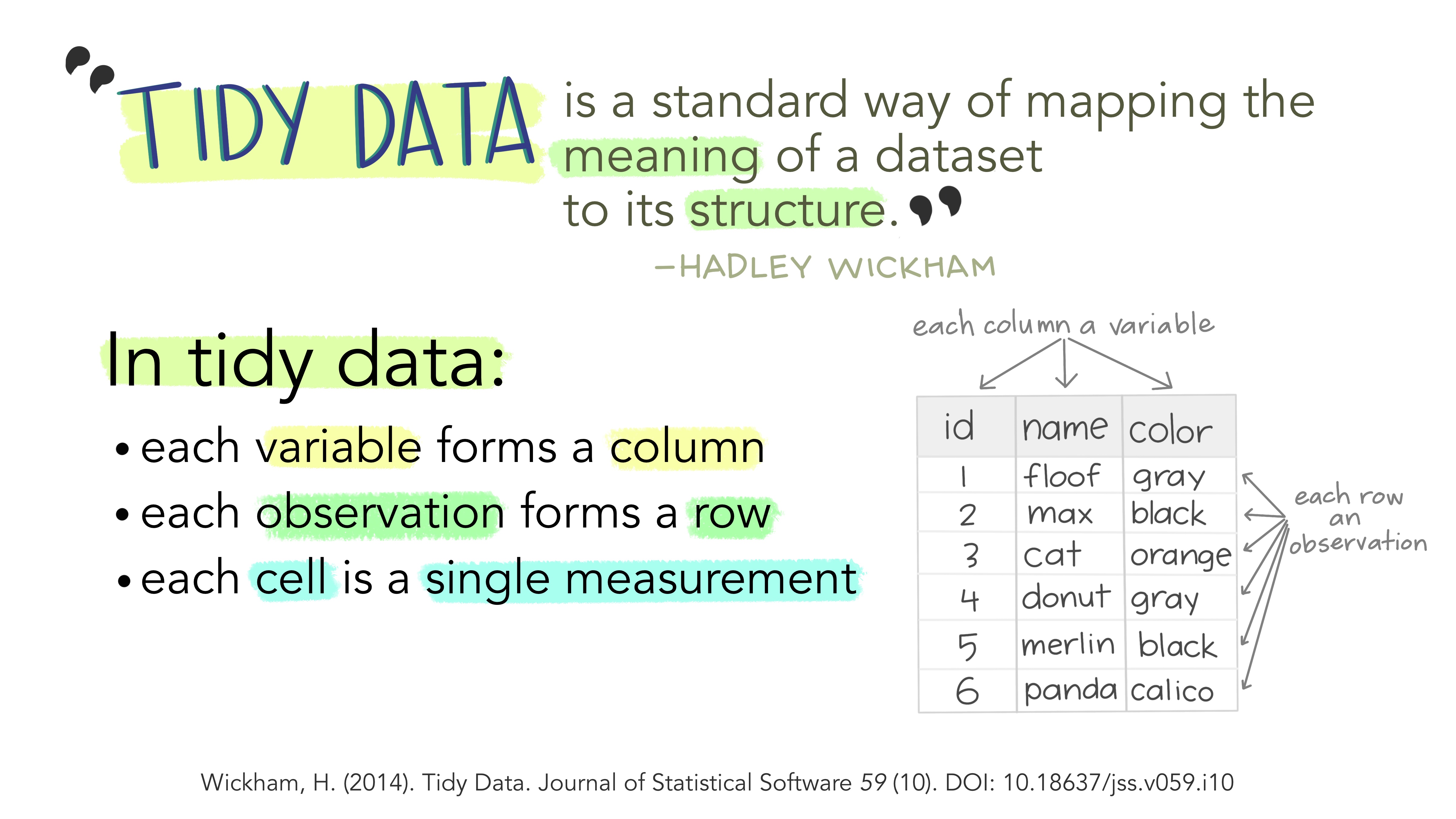
Tidy data

Structuring data is an important aspect of working with data, making it easier to analyze and visualize. The best way to work with our data is in “tidy” format.

Reshaping with `pivot_longer()` and `pivot_wider()`

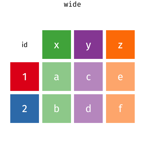
When working with tidy data there are two common dataformats for tabular datasets, wide and long.

In the example below we collected information on 3 variables – site, year, and cases.

Wide

Data relating to the same measured thing in different columns.
In this case, we have values related to our “metric” spread across multiple columns (a column each for a year).

Long

A column for each of the types of things we measured or recorded in our data.
In other words, each variable has its own column (a column for site, year, and case).

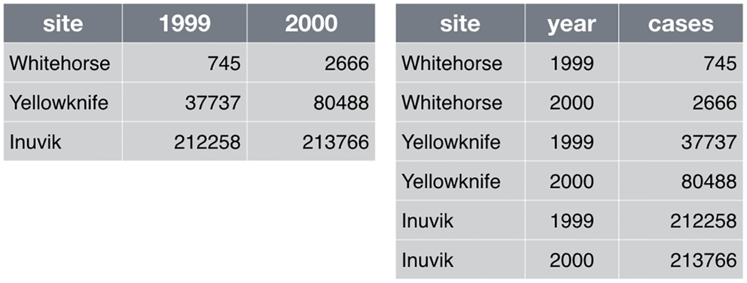
Depending on what you want do to, you might want to reshape from one form to the other. Luckily, there are functions for the pivot_wider() and pivot_longer().

Figure 3: Pivoting from wide to long formatted data. [1]

Pivoting from long to wide format

pivot_wider() takes three principal arguments

the data
the names_from column variable whose values will become new column names.
the values_from column variable whose values will fill the new column variables.

Further arguments include values_fill which, if set, fills in missing values with the value provided.

What if we wanted to plot comparisons between the weight of genera in different plots?

To do this, we’ll need to 1. Create our dataset of interest – will generate a long formatted dataframe 2. Convert from long to wide format, filling missing values with 0.

Create our dataset – use filter(), group_by() and summarize() to filter our observations and variables of interest, and create a new variable for the mean_weight.

surveys_gw <- surveys %>% 
  filter(!is.na(weight)) %>% #remove rows with empty weight
  group_by(plot_id, genus) %>% #group by plot_id and genus
  summarize(mean_weight = mean(weight)) #give me the mean weight for each group

`summarise()` has grouped output by 'plot_id'. You can override using the
`.groups` argument.

head(surveys_gw)

# A tibble: 6 × 3
# Groups:   plot_id [1]
  plot_id genus       mean_weight
    <dbl> <chr>             <dbl>
1       1 Baiomys            7   
2       1 Chaetodipus       22.2 
3       1 Dipodomys         60.2 
4       1 Neotoma          156.  
5       1 Onychomys         27.7 
6       1 Perognathus        9.62

This yields surveys_gw, a long-formatted dataframe where the observations for each plot are distributed across multiple rows, 196 observations of 3 variables.

Let’s use pivot_wider() as follows

data – the surveys_gw dataframe
names_from – genus (column variable whose values will become new column names)
values_from – mean_weight (column variable whose values will fill the new column variables)

Using pivot_wider() with the names from genus and with values from mean_weight this becomes 24 observations of 11 variables, one row for each plot.

surveys_wide <- surveys_gw %>%
  pivot_wider(names_from = genus, values_from = mean_weight, values_fill = 0)

head(surveys_wide)

# A tibble: 6 × 11
# Groups:   plot_id [6]
  plot_id Baiomys Chaetodipus Dipodomys Neotoma Onycho…¹ Perog…² Perom…³ Reith…⁴
    <dbl>   <dbl>       <dbl>     <dbl>   <dbl>    <dbl>   <dbl>   <dbl>   <dbl>
1       1    7           22.2      60.2    156.     27.7    9.62    22.2    11.4
2       2    6           25.1      55.7    169.     26.9    6.95    22.3    10.7
3       3    8.61        24.6      52.0    158.     26.0    7.51    21.4    10.5
4       4    0           23.0      57.5    164.     28.1    7.82    22.6    10.3
5       5    7.75        18.0      51.1    190.     27.0    8.66    21.2    11.2
6       6    0           24.9      58.6    180.     25.9    7.81    21.8    10.7
# … with 2 more variables: Sigmodon <dbl>, Spermophilus <dbl>, and abbreviated
#   variable names ¹Onychomys, ²Perognathus, ³Peromyscus, ⁴Reithrodontomys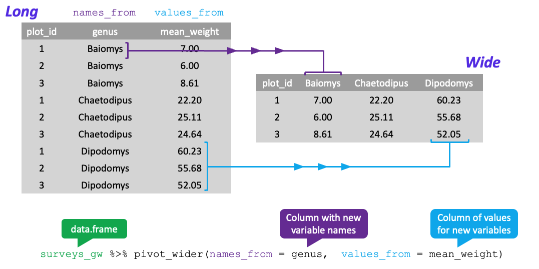

Pivoting from wide to long format

What if we wanted were given a wide format, but wanted to treat the genus names (which are column names) as values of a genus variable instead (we wanted a genus column)?

pivot_longer() takes four principal arguments:

the data
the names_to column variable we wish to create from column names.
the values_to column variable we wish to create and fill with values.
cols are the name of the columns we use to make this pivot (or to drop).

Let’s use pivot_longer() as follows

data – the surveys_wide dataframe
names_to – genus (column variable to create from column names)
values_to – mean_weight (column variable we wish to create and fill with values)
cols – -plot_id (names of columns we use to make the pivot or drop)

surveys_long <- surveys_wide %>%
  pivot_longer(names_to = "genus", values_to = "mean_weight", cols = -plot_id) #were including all cols here except plot_id

head(surveys_long)

# A tibble: 6 × 3
# Groups:   plot_id [1]
  plot_id genus       mean_weight
    <dbl> <chr>             <dbl>
1       1 Baiomys            7   
2       1 Chaetodipus       22.2 
3       1 Dipodomys         60.2 
4       1 Neotoma          156.  
5       1 Onychomys         27.7 
6       1 Perognathus        9.62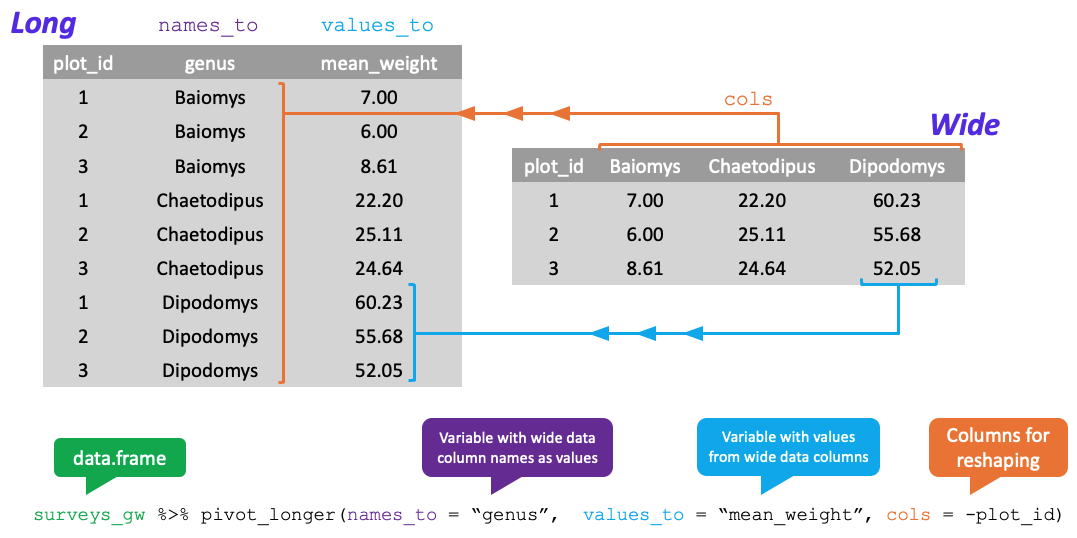

Challenge

Q&A: Reshape the surveys dataframe with year as columns, plot_id as rows, and the number of genera per plot as the values.

You will need to summarize before reshaping, and use the function n_distinct() to get the number of unique genera within a particular chunk of data. It’s a powerful function! See ?n_distinct for more.

Click here for the answer

Year is spread across columns, so we need a wide format.

each row will have a distinct plot_id
the value will be the genera per plot, for each year – which we need to calculate

surveys_wide_genera <- surveys %>%
  group_by(plot_id, year) %>% #group by plot_id and year
  summarize(n_genera = n_distinct(genus)) %>% #count number of distinct genera, create column
  pivot_wider(names_from = year, values_from = n_genera) #pivot to wide format, where names from year, and values from number of unique genera

`summarise()` has grouped output by 'plot_id'. You can override using the
`.groups` argument.

head(surveys_wide_genera)

# A tibble: 6 × 27
# Groups:   plot_id [6]
  plot_id `1977` `1978` `1979` `1980` `1981` `1982` `1983` `1984` `1985` `1986`
    <dbl>  <int>  <int>  <int>  <int>  <int>  <int>  <int>  <int>  <int>  <int>
1       1      2      3      4      7      5      6      7      6      4      3
2       2      6      6      6      8      5      9      9      9      6      4
3       3      5      6      4      6      6      8     10     11      7      6
4       4      4      4      3      4      5      4      6      3      4      3
5       5      4      3      2      5      4      6      7      7      3      1
6       6      3      4      3      4      5      9      9      7      5      6
# … with 16 more variables: `1987` <int>, `1988` <int>, `1989` <int>,
#   `1990` <int>, `1991` <int>, `1992` <int>, `1993` <int>, `1994` <int>,
#   `1995` <int>, `1996` <int>, `1997` <int>, `1998` <int>, `1999` <int>,
#   `2000` <int>, `2001` <int>, `2002` <int>

Challenge

Q&A: Now take that data frame and pivot_longer() it, so each row is a unique plot_id by year combination.

Click here for the answer

The current column values are plot_id, and a large range of years.

names_to will be year – creating a year column
values_to will be n_genera – creating a n_genera column, putting the individual cell values in this
the columns to reshape/pivot on (cols) will be the year columns, so -plot_id to select all but plot_id

surveys_long <- surveys_wide_genera %>%
  pivot_longer(names_to = "year", values_to = "n_genera", cols = -plot_id)

head(surveys_long)

# A tibble: 6 × 3
# Groups:   plot_id [1]
  plot_id year  n_genera
    <dbl> <chr>    <int>
1       1 1977         2
2       1 1978         3
3       1 1979         4
4       1 1980         7
5       1 1981         5
6       1 1982         6

Exporting data

After analyzing, processing data, we often want to export the results to a file.

Let’s create a cleaned up version of our dataset that does not include missing data (weight, hindfoot_length, and sex) – in preparation for next session.

surveys_complete <- surveys %>%
  filter(!is.na(weight),           # remove missing weight
         !is.na(hindfoot_length),  # remove missing hindfoot_length
         !is.na(sex))                # remove missing sex

We’re going to be plotting species abundances over time – so let’s remove observations for rare species (that have been observed less than 50 times).

## Extract the common species_id
species_counts <- surveys_complete %>%
    count(species_id) %>%
    filter(n >= 50)

## Use the common species id as a key for filtering (keeping)
surveys_complete <- surveys_complete %>%
  filter(species_id %in% species_counts$species_id)

To make sure that everyone has the same dataset, check the dimensions by typing dim(surveys_complete), with values matching the output shown.

dim(surveys_complete)

[1] 30463    13

Now, let’s write to a file with write_csv().

write_csv(surveys_complete, file = "~/data-carpentry/data/surveys_complete.csv")

Citations

Data Analysis and Visualization in R for Ecologists. https://datacarpentry.org/R-ecology-lesson/index.html
Wickham, H. Tidy Data. Journal of Statistical Software 59 (10). https://10.18637/jss.v059.i10

Data manipulation using dpylr and tidyr

Selecting columns and filtering rows

Connecting inputs and outputs with pipes

Challenge

Mutate

Challenge

Split-apply-combine data analysis and the summarize() function

The group_by() and summarize() functions

Counting

Challenge

Challenge

Challenge

Tidy data

Reshaping with pivot_longer() and pivot_wider()

Pivoting from long to wide format

Pivoting from wide to long format

Challenge

Challenge

Exporting data

Citations

Data manipulation using `dpylr` and `tidyr`

Split-apply-combine data analysis and the `summarize()` function

The `group_by()` and `summarize()` functions

Reshaping with `pivot_longer()` and `pivot_wider()`