dir.create("~/data-carpentry")Introduction to R and RStudio
In this initial lesson we learn the basics of R and RStudio. We begin by learning our way around RStudio and move into creating objects, writing functions, and basic data structures.
What is R? What is R Studio?
Ris a (mostly statistical) programming language and a software that interprets scripts written inRRStudiois an interface used to interact withR
Why learn R?
Increased reproducibility
When using code, your analysis can be clearly understood and easily rerun.
Increased extensibility
Combine R with 10,000+ packages to extend capabilities including image analysis, time-series, population genetics, additional languages, making websites, and more.
Works with a variety of data types, shapes, and sizes
R has special data structures and data types to handle all sorts of data.
R can also connect to spreadsheets, databases, and read in special data formats.
Can produce publication-quality graphics Base functionality and packages allow you to create a variety of graphics, while controlling minute details.
Has a large and welcoming community
The R user-community is VERY active, helpful, and welcoming.
Many resources have been developed to help people learn how to use R.
Tip
Looking for community and community resources?
Knowing your around RStudio
RStudio is an Integrated Development Environment (IDE) for working with R and can be use to do many things. We will cover things in bold and italics.
- write code and scripts
- run code
- navigate files on your computer
- inspect variables and data objects
- visualize plots
- enable version control
- develop packages
- write
Shinyapps
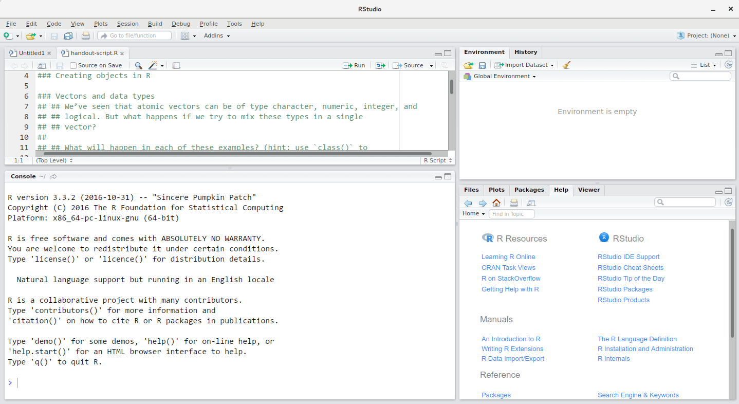
RStudio interface screenshot. Clockwise from top left: Source,Environment/History, Files/Plots/Packages/Help/Viewer,Console. [1]RStudio is divided into 4 “panes”:
- The Source for your scripts and documents (top-left, in the default layout)
- Your Environment/History (top-right) which shows all the objects in your working space (Environment) and your command history (History)
- Your Files/Plots/Packages/Help/Viewer (bottom-right)
- The
RConsole (bottom-left)
Getting Set Up
We want to keep our work (data, analyses, text) self-contained in a single directory, called the working directory. This allows us to use relative paths to other files in our scripts within that working directory so that we can move our project to other locations and share our project with others without breaking any scripts.
We can do this using “Projects” in RStudio.
- Start
RStudio. - Under the
Filemenu, click onNew Project. ChooseNew Directory, thenNew Project. - Enter a name for this new folder (or “directory”), and choose a convenient location for it. This will be your working directory for the rest of the day (e.g.,
~/data-carpentry). - Click on
Create Project. - Download the code handout, place it in your working directory and rename it (e.g.,
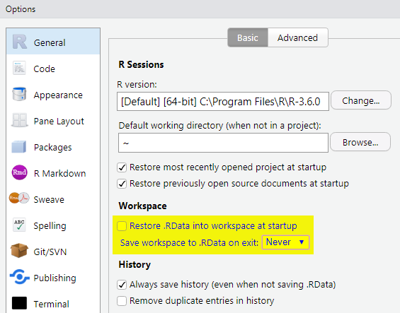
data-carpentry-script.R). - (Optional) Set Preferences to ‘Never’ save workspace in
RStudio.
Tip
Workspaces
A workspace is your working environment in R and includes any user-defined object.
By default, all objects in a workspace are saved (to .RData) and reloaded when you open your project. While this can be useful, this can result in debugging issues by having objects in memory that you forgot about. Therefore, we recommended to turn this off by
- Go to
Tools>Global Options. - Select ‘Never’ option for ‘Save workspace to .RData on exit.’
The Working Directory
The working directory is the place from there R (and your computer) will be looking for and saving files and directories.
It’s good practice to develop a common structure for your projects to:
- keep things organized
- ensure you and others can find things in various projects
- increase the portability of scripts that might be useful in multiple projects
| Directory | Contains |
|---|---|
scripts/ |
R scripts for analyses, plotting, etc. |
data/ |
Raw data and processed data (probably should be kept separately) |
documents/ |
Outlines, drafts, other texts |
Creating our directory structure
For our purposes, we’ll create the following structure
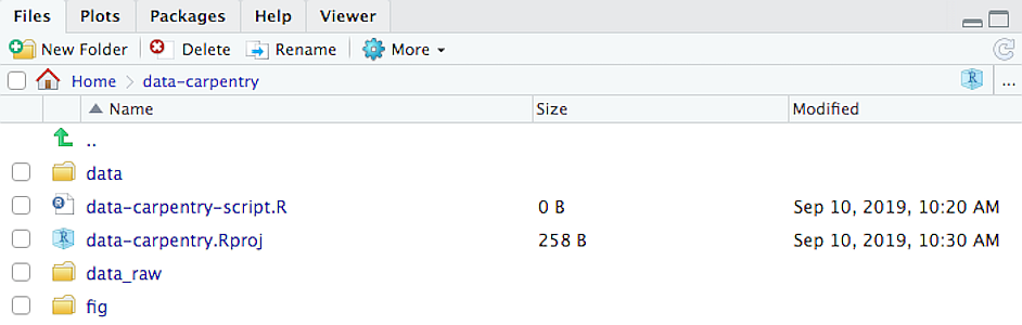
That means a working directory called data-carpentry, then 3 subdirectories, data_raw, data, and fig.
Let’s do this programmatically in the Console.
- Use
Rcommand calleddir.create, passing the value “~/data_carpentry” as the “path”.
- Create the subdirectories.
dir.create("~/data-carpentry/data_raw")
dir.create("~/data-carpentry/data")
dir.create("~/data-carpentry/fig")
Tip
The tilde ~ is a special character that means the home directory of the user.
Interacting with R
In order to do anything in R we need to tell the computer what to do. We do this with a command. An example is the dir.create command that you used to create the directory structure just now. We can do this in 2 ways
- using the console (as you did above)
- using the script pane above
What’s the benefit of using the script?
RStudio allows you to execute commands directly from the script editor.
| OS | Shortcut |
|---|---|
| Windows | Ctrl + Enter |
| macOS | Ctrl + Enter OR Cmd + Return |
You can find other keyboard shortcuts in this RStudio cheatsheet about the RStudioIDE.
Seeking help
If you need help with a specific function, for instance mean(), you can type ?mean() and press enter. Documentation on the function will pop up in the Help window.

RStudio help panel. When typing a word in the search field, it will show related suggestions. [1]Automatic Code Completion
When you write code in RStudio, you can use its automatic code completion to remind yourself of a function’s name or arguments.
- Start typing the function name and pay attention to the suggestions that pop up.
- Use the up and down arrow to select a suggested code completion and Tab to apply it.
Tip
You can also use code completion to complete function’s argument names, object, names and file names. It even works if you don’t get the spelling 100% correct.
Dealing with error messages
We WILL encounter errors, and a lot of them! Watch for red “X”’s next to the line number in RStudio to catch them.
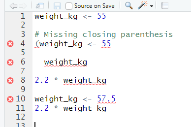
RStudio shows a red x next to a line of code that R doesn’t understand. [1]If you need more help
- Google the error
- Ask a question (with appropriate context and an example) on Stack Overflow
Creating objects in R
You can get output from R simply by typing math in the console:
3 + 5[1] 812 / 7[1] 1.714286This can be more useful if we store these values as objects, which would allow us to refer back to these objects later.We do this by using the assignment operator <-.
For example, if we wanted to create an object named weight_kg and assign it the value of 55, we could type the following
weight_kg <- 55
Note
A note on naming
Objects can be named just about anything (x, the_thing, other_5tUfF). Be thoughtful about what you use. Below are some guidelines
- Be explicit and not too long.
- They cannot start with a number (
2xis not valid, butx2is). - R is case sensitive, so for example,
weight_kgis different fromWeight_kg. - There are some names that cannot be used because they are the names of fundamental functions in
R(e.g.,if,else,for, see here for a complete list). If in doubt, double-check - Avoid dots (
.) within names. Dots have a special meaning (methods) inRand other programming languages. To avoid confusion, don’t include dots in names. - Use nouns for object names and verbs for function names.
- Be consistent in the styling of your code, such as where you put spaces, how you name objects, etc.
When assigning a value to an object, R does not print anything. You can force R to print the value by using parentheses or by typing the object name:
weight_kg <- 55    # doesn't print anything
(weight_kg <- 55)  # but putting parenthesis around the call prints the value of `weight_kg`
[1] 55weight_kg # and so does typing the name of the object[1] 55Now that R has weight_kg in memory, we can do arithmetic with it. Let’s convert this weight into pounds (weight in pounds is 2.2 times the weight in kg):
2.2 * weight_kg[1] 121We can also change an object’s value by assigning it a new one:
weight_kg <- 57.5
2.2 * weight_kg
[1] 126.5Assigning a value to one object does not change the values of other objects.
For example, let’s store the animal’s weight in pounds in a new object, weight_lb:
weight_lb <- 2.2 * weight_kgNow, let’s change weight_kg to 100.
weight_kg <- 100What do you think is the current content of the object weight_lb? 126.5 or 220?
Saving your code
Until now, we’ve used the console. Since we want to save our work, let’s
- Open up a script – by pressing Ctrl + Shift + N.
- Save the script – by pressing Ctrl + S and selecting the save location, and naming it.
Adding Comments
In R the comment character is #. Anything to the right of # in a script will be ignored by R. We use comments to leave notes and explanations in scripts.
Challenge
Q&A: What are the values after each statement in the following?
mass <- 47.5            # mass?
age  <- 122             # age?
mass <- mass * 2.0      # mass?
age  <- age - 20        # age?
mass_index <- mass/age # mass_index?Functions and their arguments
Functions are “canned scripts” that automate more complicated sets of commands including operations assignments, etc.
- Usually takes one or more inputs called arguments
- Often return a value (but not always)
- Example:
sqrt()takes a number as the argument and returns the square root of the number
Note
Many functions are predefined, or can be made available by importing R packages (more on that later).
Executing a function (‘running it’) is called calling the function. An example of a function call is:
weight_kg <- sqrt(10)Let’s break it down
- the value of 10 is given to the
sqrt()function - the
sqrt()function calculates the square root - the function returns the value which is then assigned to the object
weight_kg
Return values
As noted earlier, a value is not always returned. If returned, the return ‘value’
- can be any value, or thing
- can be multiple values (a set of things)
- can even be a dataset
Arguments
Arguments can be anything, not only numbers or filenames, but also other objects.
- Each argument can differ based on the function, and must be looked up in the documentation (see below).
- Some functions take multiple arguments
- Some arguments MUST be specified by the user when calling the function
- Some arugments might take on a default value (these are called options) if left out
Tip
Options are typically used to alter the way the function operates, such as whether it ignores ‘bad values’, or what symbol to use in a plot. However, if you want something specific, you can specify a value of your choice which will be used instead of the default.
Let’s try a function that can take multiple arguments: round().
round(3.14159)[1] 3We called round() with just one argument, 3.14159, and it returned the value 3. That’s because the default is to round to the nearest whole number.
Let’s modify the number of digits we want in the answer. How do we know how to find more information about the round function?
We can use args(round) to find what arguments it takes.
args(round)function (x, digits = 0)
NULLWe can also look at the help for this function using ?round.
?roundWe see that if we want a different number of digits, we can type digits = 2 or however many we want. Let’s try it.
round(3.14159, digits = 2)[1] 3.14If you provide the arguments in the exact same order as they are defined you don’t have to name them:
round(3.14159, 2)[1] 3.14And if you do name the arguments, you can switch their order:
round(digits = 2, x = 3.14159)[1] 3.14
Tip
It’s good practice to put the non-optional arguments (like the number you’re rounding) first in your function call, and to then specify the names of all optional arguments. If you don’t, someone reading your code might have to look up the definition of a function with unfamiliar arguments to understand what you’re doing.
Vectors and data types
A vector is the most common and basic data type in R.
- Can be a series of values (numbers or characters).
- Assigned using
c()function
For example, let’s create a vector of animal weights and assign it to an object weight_g:
weight_g <- c(50, 60, 65, 82)
weight_g
[1] 50 60 65 82A vector can also contain characters:
animals <- c("mouse", "rat", "dog")
animals
[1] "mouse" "rat" "dog" The quotes around “mouse”, “rat”, etc. are essential here. Without the quotes R will assume objects have been created called mouse, rat and dog. As these objects don’t exist in R’s memory, there will be an error message.
There are many functions that allow you to inspect the content of a vector. length() tells you how many elements are in a particular vector:
length(weight_g)[1] 4length(animals)[1] 3All of the elements are the same type of data. The function class() indicates what kind of object you are working with:
class(weight_g)[1] "numeric"class(animals)[1] "character"The function str() provides an overview of the structure of an object and its elements. It is a useful function when working with large and complex objects:
str(weight_g) num [1:4] 50 60 65 82str(animals) chr [1:3] "mouse" "rat" "dog"You can use the c() function to add other elements to your vector:
weight_g <- c(weight_g, 90) # add to the end of the vector
weight_g <- c(30, weight_g) # add to the beginning of the vector
weight_g
[1] 30 50 60 65 82 90Let’s break this down:
- In the first line, we take the original vector
weight_g, add the value90to the end of it, and save the result back intoweight_g. - Then we add the value
30to the beginning, again saving the result back intoweight_g.
We can do this over and over again to grow a vector, or assemble a dataset. As we program, this may be useful to add results that we are collecting or calculating.
An atomic vector is the simplest R data type and is a linear vector of a single type. These are the basic building blocks that all R objects are built from.
The there are 6 main atomic vector thar R uses:
"character"for character (A) or string values (Apple)"numeric"(or"double") for all real numbers with our without decimal values"logical"forTRUEandFALSE(the boolean data type)"integer"for integer numbers (e.g.,2L, theLsuffix indicates toRthat it’s an integer)"complex"to represent complex numbers with real and imaginary parts (e.g.,1 + 4i) and that’s all we’re going to say about them"raw"for bitstreams that we won’t discuss further
You can check the type of your vector using the typeof() function and inputting your vector as the argument.
Vectors are one of the many data structures that R uses. Other important ones are lists (list), matrices (matrix), data frames (data.frame), factors (factor) and arrays (array).
Challenge
Q&A: What happens if we try to mix these types in a single vector?
Q&A: What will happen in each of these examples? (hint: use class() to check the data type of your objects):
num_char <- c(1, 2, 3, "a")
num_logical <- c(1, 2, 3, TRUE)
char_logical <- c("a", "b", "c", TRUE)
tricky <- c(1, 2, 3, "4")Q&A: Why do you think it happens?
Q&A: How many values in combined_logical are "TRUE" (as a character) in the following example (reusing the 2 ..._logicals from above):
combined_logical <- c(num_logical, char_logical)Q&A: You’ve probably noticed that objects of different types get converted into a single, shared type within a vector. In R, we call converting objects from one class into another class coercion. These conversions happen according to a hierarchy, whereby some types get preferentially coerced into other types. Can you draw a diagram that represents the hierarchy of how these data types are coerced?
Subsetting vectors
If we want to extract one or several values from a vector, we must provide one or several indices (positions of elements in the object, starting with 1) in square brackets.
For instance:
animals <- c("mouse", "rat", "dog", "cat")
animals[2]
[1] "rat"animals[c(3, 2)][1] "dog" "rat"We can also repeat the indices to create an object with more elements than the original one:
more_animals <- animals[c(1, 2, 3, 2, 1, 4)]
more_animals
[1] "mouse" "rat" "dog" "rat" "mouse" "cat" R indices start at 1. Programming languages like Fortran, MATLAB, Julia, and R start counting at 1, because that’s what human beings typically do. Languages in the C family (including C++, Java, Perl, and Python) count from 0 because that’s simpler for computers to do.
Conditional subsetting
Another common way of subsetting is by using a logical vector.
TRUEwill select the element with the same indexFALSEwill not select the element with the same index
weight_g <- c(21, 34, 39, 54, 55)
weight_g[c(TRUE, FALSE, FALSE, TRUE, TRUE)]
[1] 21 54 55Some functions and logical tests will output vectors of logical values, which can be useful.
For exmaple, if you wanted to select only the values above 50:
weight_g > 50 # will return logicals with TRUE for the indices that meet the condition[1] FALSE FALSE FALSE TRUE TRUE## so we can use this to select only the values above 50
weight_g[weight_g > 50][1] 54 55Let’s break it down. 1. The weight_g > 50 inside the brackets is evaluated and returns a list of TRUE for indices less than 50 2. The outside weight_g is subsetted based on that returned list, pulling out only the indices that are TRUE
You can combine multiple tests using & (both conditions are true, AND) or | (at least one of the conditions is true, OR):
weight_g[weight_g > 30 & weight_g < 50][1] 34 39weight_g[weight_g <= 30 | weight_g == 55][1] 21 55weight_g[weight_g >= 30 & weight_g == 21]numeric(0)A quick overview of some operators
| Operator | Meaning |
|---|---|
& |
and |
| |
or |
> |
greater than |
< |
less than |
>= |
greater than or equal to |
<= |
less than or equal to |
== |
is equal to |
The function %in% allows you to test if any of the elements of a search vector are found:
animals <- c("mouse", "rat", "dog", "cat", "cat")

# return both rat and cat
animals[animals == "cat" | animals == "rat"]
[1] "rat" "cat" "cat"# return a logical vector that is TRUE for the elements within animals
# that are found in the character vector and FALSE for those that are not
animals %in% c("rat", "cat", "dog", "duck", "goat", "bird", "fish")[1] FALSE TRUE TRUE TRUE TRUE# use the logical vector created by %in% to return elements from animals
# that are found in the character vector
animals[animals %in% c("rat", "cat", "dog", "duck", "goat", "bird", "fish")][1] "rat" "dog" "cat" "cat"Challenge
Q&A: Can you figure out why "four" > "five" returns TRUE?
Missing data
Missing data are represented in vectors as NA. When doing operations on numbers, most functions will return NA if the data you are working with include missing values.
For example, the mean() below:
heights <- c(2, 4, 4, NA, 6)
mean(heights)
[1] NAThis feature makes it harder to overlook the cases where you are dealing with missing data. You can add the argument na.rm = TRUE to calculate the result as if the missing values were removed (rm stands for ReMoved) first.
heights <- c(2, 4, 4, NA, 6)
mean(heights, na.rm = TRUE)
[1] 4If your data include missing values, you may want to become familiar with the functions is.na(), na.omit(), and complete.cases(). See below for examples.
## Extract those elements which are not missing values.
heights[!is.na(heights)]
[1] 2 4 4 6## Returns the object with incomplete cases removed.
#The returned object is an atomic vector of type `"numeric"` (or #`"double"`).
na.omit(heights)[1] 2 4 4 6
attr(,"na.action")
[1] 4
attr(,"class")
[1] "omit"## Extract those elements which are complete cases.
#The returned object is an atomic vector of type `"numeric"` (or #`"double"`).
heights[complete.cases(heights)][1] 2 4 4 6Recall that you can use the typeof() function to find the type of your atomic vector.
Challenge
Q&A: 1. Using this vector of heights in inches, create a new vector, heights_no_na, with the NAs removed.
heights <- c(63, 69, 60, 65, NA, 68, 61, 70, 61, 59, 64, 69, 63, 63, NA, 72, 65, 64, 70, 63, 65)Use the function
median()to calculate the median of theheightsvector.Use
Rto figure out how many people in the set are taller than 67 inches.?
Citations
- Data Analysis and Visualization in R for Ecologists. https://datacarpentry.org/R-ecology-lesson/index.html