The most crucial step when setting up your own app is curating your data in preparation for loading into the browser. There are two reasons for these steps:
- formatting the data into
AnnDatafiles, which creates a database accessible by the browser - identifying the variables (i.e., columns in a table) that will be browsable, which specifies how data can be selected and/or manipulated in the browswer interface
As the Curator you have the responsibility to understand the specific research questions involved in your data, and how to allow these questions to be explored using a visualization tool.
The process of curating your data generally includes the following steps:
-
Format and ingest raw data - translate the outputs of your experimental data (post-QC phase) into scanpy’s
AnnDatastructure - Post-processing - create additional columns and fields of interest. E.g. dimension reduction, compute relevant marginal quantities, define additional annotation and grouping variables, etc.
- Differential expression tables - compute and/or format existing tables of the different expression levels relative to experimental conditions
-
Write database - write the data and configuration files to a named directory which we will define as a database.
-
database context documentation - define the context and for the dataset. This involves editing/creating the R-markdown file which will render in the browser app (
additional_info.Rmd)
Each step of data curation is generally described below, referencing the PBMC3k dataset from 10X Genomics as an example. The complete script used for curation can be found in examples/browse_pbmc3k.R. Additional examples of how the data curation process is applied to various data types and use cases can be found in the examples/ subdirectory.
Data organization
There are three main locations you’ll need to specify while curating your data and otherwise preparing your browser app:
-
run directory: location from which the browser is launched. For the PBMC3k example, we will refer to this as
OMICSER_RUN_DIR, and create a new directory namedomicser_test/which will contain the other content for this project. If you plan to make more extensive modifications to the browser, we recommend cloning theomicserpackage and using the top level folder for your run directory. -
location of data: folder containing your -omics data, referred to as
RAW_DIRand set toraw_data/in the PBMC3k example. This location is only used in the data curation steps. -
location of database: folder containing the formatted data produced by the data curation steps, packaged to be ingested for visualization in a browser. For the PBMC3k example, it is referred to as
DB_ROOT_PATHand set astest_db/we will be working with a single dataset (and single dataset), though it is possible to visualize multiple datasets with the same browser configuration (i.e., this folder can potentially contain multiple databases).
Example data from 10X Genomics
The example data used for this tutorial are from ~3000 peripheral blood mononuclear cells (PBMCs) from a healthy donor. Further information about the data is available at the 10X Genomics website. These data have also been used in tutorials from scanpy and Seurat.
The PBMC3k example script includes code sections to help you install software/environments, download/organize data, and otherwise prepare for the data curation steps below. Please note that the data files from 10X Genomics need to be saved as .gz files for them to be read correctly when importing the data.
2. Format and ingest raw data
The exact steps required to ingest raw data vary widely depending on your data type and how these data are formatted. The general goal is to obtain the data necessary to create an AnnData object containing all data and metadata required for visualization.
AnnData Schema
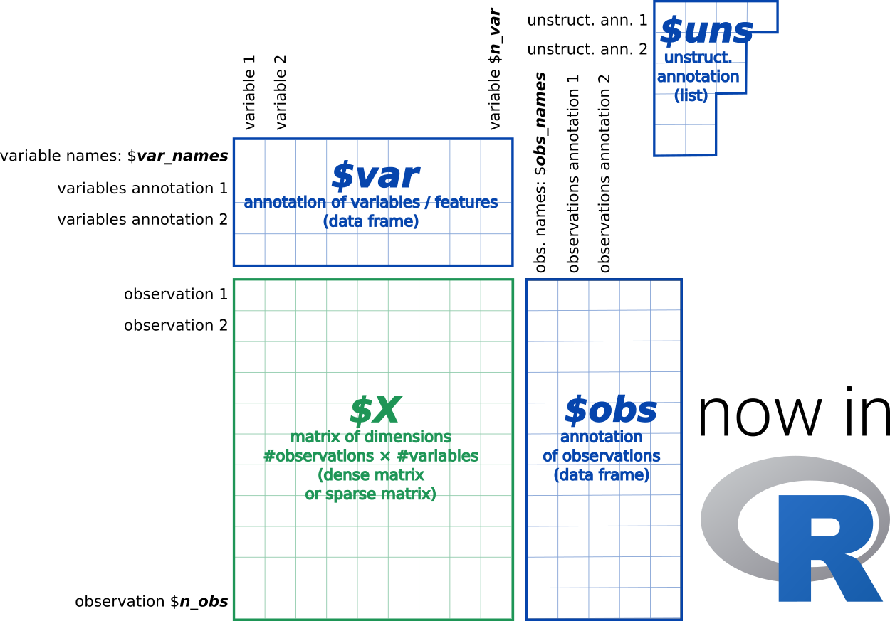
The AnnData format includes three types of data:
- DATA ($X): a matrix of measurements - e.g. count matrix of cells by genes (for transcriptomic data).
-
FEATURE METADATA ($var): a table of
omicannotation - e.g. gene/protein names, families, “highly variable genes”, “is marker gene”, etc. - SAMPLE METADATA ($obs): a table of sample annotations - e.g. cell types, sample #, batch ID sex, experimental condition, etc.
More information on this format is available on the AnnData for R website.

 ### Ingesting raw data
For our example, we’ll read the PBMC3k data files using the read_10x_mtx() function from Python’s scanpy package, then writing the data to file in .h5ad format. We’ll access scanpy using the reticulate R package. If you have difficulty accessing scanpy in this section,please see the troubleshooting section below.
Please see the other example curation scripts to understand how other data can be processed at this step. This may include writing custom helper scripts to standardize data manipulation from files resulting from your data generation processes.
Formatting as AnnData
Our next step will use the raw database we just created and add the consistent structure we’ll need to orient the browser features later. The omicser::setup_database() function incorporates the three separate data sources (DATA matrix, omic FEATURE METADATA annotations, and SAMPLE METADATA) into the AnnData object.
For our PBMC3k example, we’ll apply the omicser::setup_database() function:
# identify location of raw data
data_list <- list(object = path(DB_ROOT_PATH, DB_NAME, "core_data.h5ad"))

# create database formatted as AnnData
adata <- omicser::setup_database(database_name = DB_NAME,
                                 db_path = DB_ROOT_PATH,
                                 data_in = data_list,
                                 re_pack = TRUE)
In this case, all data necessary was ingested in the previous step. This results in a database that is consistently formatted, and thus able to potentially be combined with other datasets in the future.
3. Post-processing
Now that the data are packed into the the AnnData object, we can leverage additional functions from scanpy via reticulate to do perform additional data post-processing. The for the PMBC3k data includes steps to filter, annotate, and otherwise prepare the data for visualization. The data are periodically saved at intermediate steps, which is useful for optimizing visualizations. such as dimension reduction and clustering.
You have flexibility in the data curation process regarding which approaches you use, and when those steps are performed. For example, clustering and dimension reduction isn’t required to browse data, but is a useful step if you’d like to work with your data in other tools, like
cellxgene.
The example below demonstrates a semi-automatic procedure to infering clusters in the data using the scanpy python library for processing AnnData data. For more information on using scanpy in R, please see the troubleshooting section below.
4. Create differential expression tables
The ability to identify which -omics features differ among categories is perhaps the most important part of data curation. However, it is also one of the trickiest parts, as some data generation services (especially for proteomics) compute differential expression (DE) using commercial software associated with instrumentation. These algorithms leverage bespoke statistics, with unknown assumptions about the statistical tests involved, so it will be best to reformat those tables. Additionally, the schema below provides a way to standardize comparisons across datasets, which is important for browsers drawing from multi-omics data.
DE Table Schema
The differential expression table has the following fields:
-
group- the comparison, using the format {names}V{reference} from fields below -
names- what are we comparing? -
obs_name- name of the metadata variable -
test_type- what statistic are we using? -
reference- the denominator, or the condition against which we are comparing expressions values -
comp_type- same format asgroup, as grpVref or grpVrest, with rest representing all other conditions -
logfoldchanges- log2(name/reference) -
scores- statistic score -
pvals- pvalues from the statisticals test, e.g. t-test -
pvals_adj- adjusted pvalue (Q) -
versus- label which we will choose in the browser
Computing the DE table
The omicser::compute_de_table() leverages scanpy functions and the AnnData object to compute differential expression and provide a properly formatted DE table. We will need to provide the function with the following parameters:
-
adata- the anndata object -
comp_types- what kind of comparisons? there are two types:- “allVrest” which takes each of our experimental conditions in turn and compares against the “rest” of the data.
- “{a}V{b}” or “firstgroupVsecondgroup” which compares the experimental condition “firstgroup” against “secondgroup”
-
test_types- statistical tests. See our examples orscanpydocumentation for which test types are available. -
obs_names- name of theadata$obscolumn defining the comparision groups -
sc- the scanpy data object we imported withreticulate
Here’s an example which computes a differential expression with a wilcoxon test of significance for each of our inferred groups (leiden) with respect to the rest of the groups. (These groups were inferred programmically via dimension reductions and a “leiden” clustering procedure via Scanpy tools.cf line 207 of pbmc3k_curate_and_config.R)
sc <- reticulate::import("scanpy")
test_types <- c('wilcoxon')
comp_types <- c("grpVrest")
obs_names <- c('leiden')
diff_exp <- omicser::compute_de_table(adata,comp_types, test_types, obs_names,sc)
The DE table output from this function should be saved to the database folder as db_de_table.rds:
5. Write database
The last step of data curation is to write the final database to the database directory as db_data.h5ad:
adata$write_h5ad(filename=file.path(DS_ROOT_PATH,DB_NAME,"db_data.h5ad"))At this point, each folder in your database directory should include at least three files. Shiny will look for these files when creating the browser, so their names and location are important:
-
db_data.h5ad- theAnnDataobject
-
db_de_table.rds- differntial expression table 3,additional_info.Rmd- expository explanation of the context and logic of database
You may also have intermediate database files created during post-processing: normalized_data.h5ad,core_data.h5ad,and norm_data_plus_dr.h5ad. They are available for your reference, but are not required for further app development.
Now that the data are formatted and organized appropriately, we’ll continue to the next step and configure the browser.
6. Documenting the data and analysis
It is useful, and in many cases necessary, to include information about your data and analysis methods when sharing a visualization tool with your colleagues. This section describes approaches for sharing such information within the browser application.
database context
The box on the right of the Ingest tab in the browser application is available for documenting both analysis methods (pre-processing approaches/assumptions, hypotheses being tested, statistical parameters) as well as information about the project (link to preprint/publication, acknowledgements, etc).
The content of this tab is rendered from additional_info.Rmd. If you choose to customize this file, you must organize your browser application files within a copy (clone) of the omicser. This ensures that your modified copy of additional_info.Rmd is read when you launch your browser, instead of the original version from your installed library.
Troubleshooting
scanpy in R
If you have difficulty accessing scanpy, please see the Troubleshooting section of 1-Installation
scanpy was originally written as a Python package, but we are using it within R courtesy of the reticulate R package. The original scanpy documentation can help you understand the assumptions and requirements of functions, which retain the same names between Python and R. For more information on syntax for scanpy in R, please see this documentation.